3d. Presentations
4. Acknowledgements
5. References
Tables
Table 1. CTD Station Information
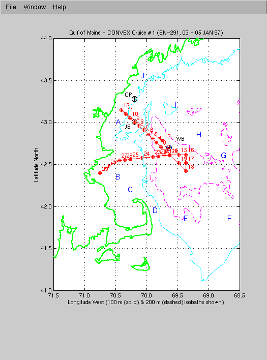
Figure 1. EN291 CTD station locations. CTD stations and UNH mooring
sites are marked. Stations are numbered sequentially.
An ASCII listing of the CTDs
is available.
Figure 2. Wilkinson Basin 1997 mooring configuration.
Figure 3. CTD salinity calibration plots.
Figure 4. Composite of EN291 CTD profiles.
Figure 5.a. Hydrography section A to F (stations 12 to 02, 20 to 18):
vertical sections of temperature, salinity, and sigma theta.
Figure 5.b. Hydrography section B to G (stations 29 to 21, 14 to 16):
vertical sections of temperature, salinity, and sigma theta.
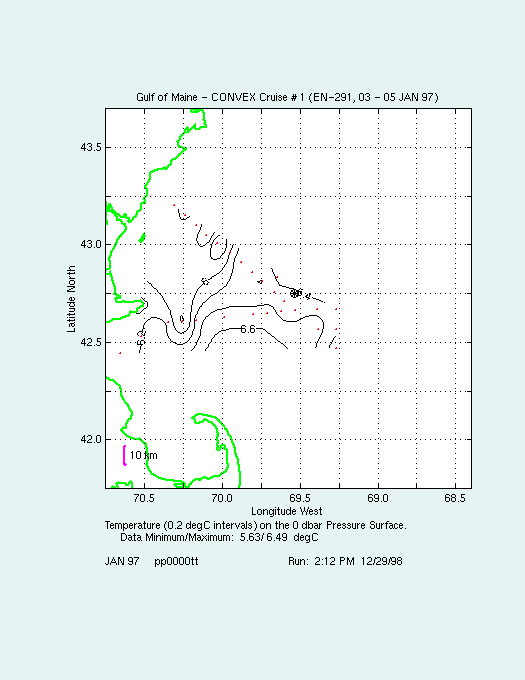
Figure 6.a. Contours of the observed temperature on the ocean surface.
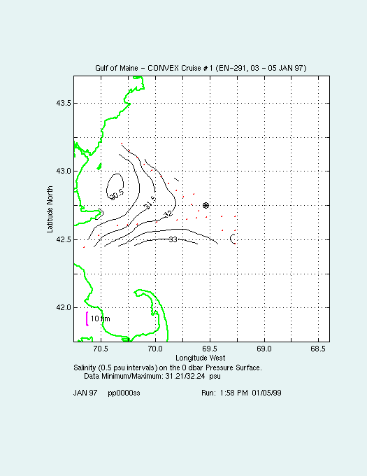
Figure 6.b. Contours of the observed salinity on the ocean surface.
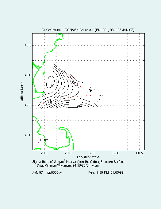
Figure 6.c. Contours of the observed density on the ocean surface.
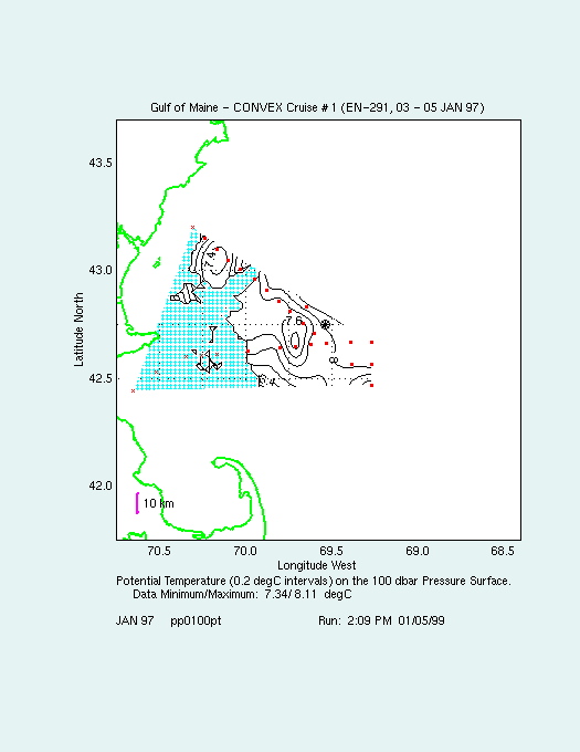
Figure 7.a. Contours of the observed temperature on the 100 dbar surface.
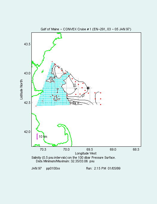
Figure 7.b. Contours of the observed salinity on the 100 dbar surface.
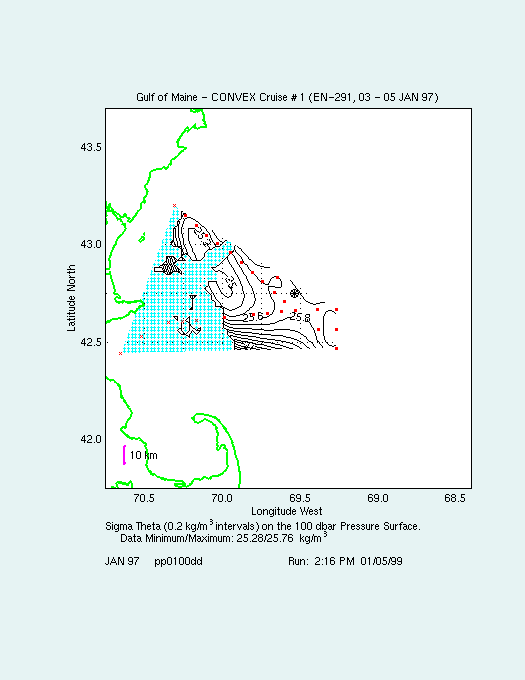
Figure 7.c. Contours of the observed density on the 100 dbar surface.
Figure 8. Contours of the sigma theta 26.00 density surface depth.
Appendix Figures
Individual profiles at each hydrographic station are available for viewing on 2 pages:
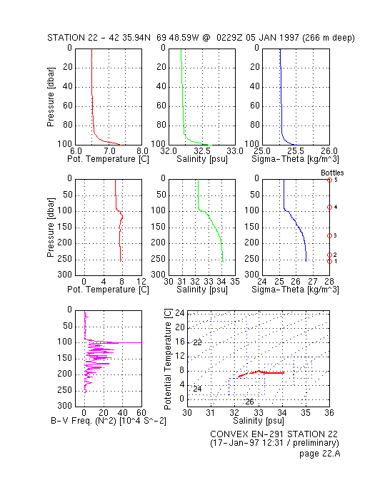
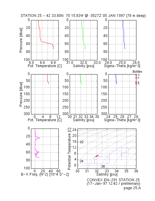
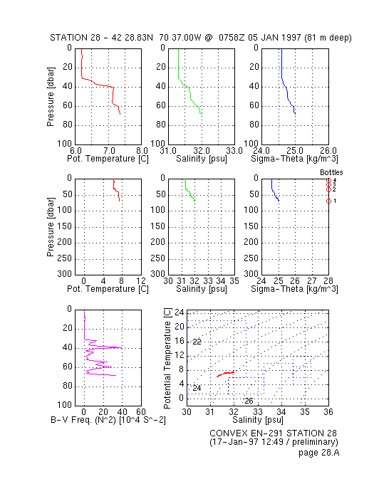
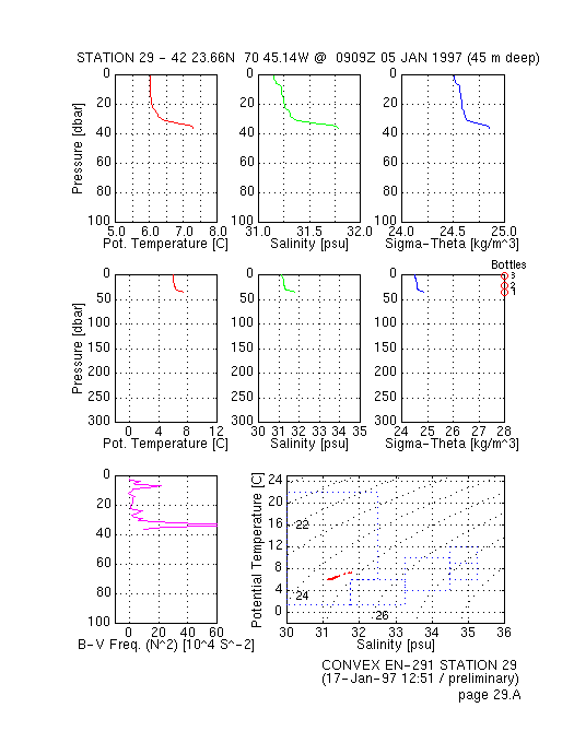
Page A: Station profiles of temperature, salinity, sigma-theta density, stability (N-squared),
and temperature-salinity diagram (top 3 panels show surface layer profiles at higher resolution, the
remaining panels are all on the same depth /property scale for intercomparison).
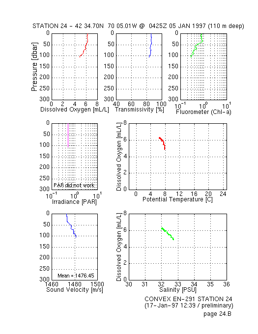
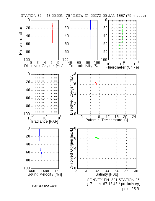
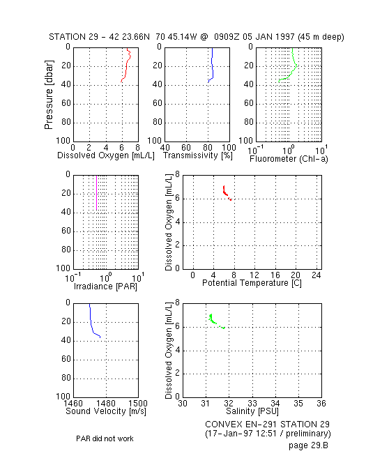
Page B: Station profiles of dissolved oxygen, transmissivity, fluorometer (Chl-a), irradiance (PAR),
temperature-dissolved oxygen, and salinity-dissolved oxygen diagrams when observed.
Leg A Stations:
02A,
02B,
03A,
03B,
04A,
04B,
05A,
05B,
06A,
06B,
07A,
07B,
08A,
08B,
09A,
09B,
10A,
10B,
11A,
11B,
12A,
12B,
13A,
13B,
18A,
18B,
19A,
19B,
20A,
20B.
Leg B Stations:
14A,
14B,
15A,
15B,
16A,
16B,
21A,
21B,
22A,
22B,
23A,
23B,
24A,
24B,
25A,
25B,
26A,
26B,
27A,
27B,
28A,
28B,
29A,
29B.
This report describes the hydrographic measurements obtained 3-5 January 1997, as part of the
NSF-supported "Observational / Modeling Study of Wintertime Convection and Water Mass Formation"
in the western Gulf of Maine (GOM). Herein we document the first of seven planned University of
New Hampshire (UNH) cruises aboard the R/Vs ENDEAVOR and OCEANUS as part of this "Convective
Overturn Experiment" (CONVEX). This report and these data can be accessed via the WWW address:
http://ekman.sr.unh.edu/OPAL/CONVEX/
1. Introduction
Wintertime atmospherically forced convective overturning (and subsequent mixing) is responsible
for significant deep water formation in the Greenland Sea, the Labrador Sea, the western Mediterranean,
and the Arctic / Antarctic polar regions. Observational evidence suggests that related water mass
formation processes are also active in the Gulf of Maine during wintertime.
In this project, the GOM is being used as a convenient environmental laboratory to explore the physics
of overturning and mixing with an integrated program of observation and modeling. The research will
address basic questions concerning the kinematics and energetics of mixed layer formation in winter,
with an emphasis on water column convective instability, sinking, and mixing in the presence of
strong wind stress and surface cooling.
As the observations cannot resolve all the scales of this process, they will be integrated with the
results of a numerical non-hydrostatic Ocean Large Eddy Model (OLEM) to provide further insight into
the role of small-scale convection in wintertime water mass formation.
Field experiments, consisting of moored array and hydrographic / ADCP observations and augmented by
hydrographic surveys, operational meteorological data and satellite imagery, are being conducted during
the winters of 1996-97 and 1997-98.
The first year's experiment will be in shallower coastal water (near Jeffreys Basin-JB) where the convective
plumes interact with the bottom. During the first and second year, experiments will also be conducted in
deeper offshore water (central Wilkinson Basin-WB) where convective activity does not reach the bottom.
A central temperature / conductivity chain, two adjacent temperature chains, bottom pressure sensors,
and ADCP vertical velocity measurements will provide both temporal and spatial information on the form
and frequency of small scale convective plumes and mixed layer structure changes. Additional basin-scale
information will be derived from hydrographic surveys (as reported here), regional land and buoy weather
observations, and satellite SST imagery.
These data will be used to assess the fidelity of the results from a series of OLEM experiments, designed
to (a) model "typical" convective plumes and (b) determine the relative importance of convection and wind
mixing in the water mass formation process. The observations will also be used to relate the patterns and
intensity of convective overturning to winter mixed layer structure and water mass formation.
1.a. Moored Observations
The 1996-7 CONVEX field observation program consists of the wintertime deployment of moored current /
conductivity / temperature / bottom pressure instrumentation (Figure 2) and
a series of hydrographic transects (Figure 1). During January 1997, a moored
array was deployed in the center of Wilkinson Basin (Figure 2). A coastal pressure
sensor was also deployed at the Coast Guard pier on Newcastle Island in Portsmouth Harbor, NH. These pressure
sensors will provide across-shelf pressure difference fluctuations which are proportional to along-shelf
geostrophic currents. The velocity / temperature / conductivity measurements will resolve the hourly changes
in the physical properties of the water at several depths at the moorings.
1.b. Hydrographic Surveys
Hydrographic profile measurements will provide relatively high (spatial) resolution water property information
along transects through WB and include the WB and JB moored measurements (Figure 1).
The combination of the time series data from the moorings and the spatial data from the hydrographic cruises
will help us to understand the characteristics of wintertime water mass formation in the vicinity of the moorings
and the along-coast currents in the western GOM.
2. Cruise Narrative
The R/V Endeavor departed the Naval Station Newport, RI pier at midnight local (0500Z) 3 January 1997,
and passed through the Cape Cod Canal enroute to Wilkinson Basin. Beginning approximately 1200L (1700Z)
3 January 1997, oceanographic mooring WB-97 (Figures 1 and 2) was set. The anchor for the mooring was released
at 1323L (1823Z) near 42° 36.82'N 69° 37.64' W in 277 m of water. The deployed instrument string included
temperature, conductivity and current velocity sensors at nominal depths of 42, 140 and 230 m (Figure 2) and a VACM current meter at 40 m. A bottom instrument package containing a pressure and
temperature sensor was released nearby at 1338L (1838Z) near 42° 36.85'N 69° 37.60' W.
After a CTD profile was observed at the mooring site, using the Endeavor SeaBird SBE-911+ (measuring
pressure, temperature, conductivity, dissolved oxygen, fluorescense, PAR and light transmission), two
hydrographic lines were surveyed (Figure 1): (Leg A) 15 stations bearing
northwestward between WB-97 and point A off the New Hampshire coast and (Leg B) 12 stations bearing
westward between WB-97 and the vicinity of Boston, MA. Three CTD profiles were observed at the WB-97 site
to produce a short 'time series,' making a total of 28 good CTD profiles. Up to 6 Niskin bottle samples
were taken at each site for nutrient analyses (T. Loder, UNH) and oxygen isotope studies (R. Houghton, LDOI).
On 4 January, the bathymetry near 42° 46.92' N 69° 44.85' W was surveyed and we dragged for a lost
mooring and instrument set from a 21 March 1994 deployment, with no luck.
Two drifting buoys (10 and 40 m depths) were released at 1615L at 42° 37.00'N 68 deg 35.5' W
(for R. Limeburner, WHOI). While underway, ship instruments routinely recorded near-surface temperature /
salinity and a weather instrument package (IMET) provided a continuous records of air pressure, temperature,
relative humidity, wind speed / direction, short / long wave radiation, along with ship's position and movement.
A RDI 150 KHz Acoustic Doppler Current Profiler (ADCP) recorded ocean current structure along the ship's path.
At 0420L 5 January, the final CTD was completed and the ship started for home via the Cape Cod Canal.
We tied up at 1400L at the pier on Naval Station Newport.
Postlog: On 8 January 1997, we learned that our buoy was no longer in place- it had lasted
less than 5 days. The pressure sensor platform was later dragged up by a fisherman and returned to us during
February 1997. Late summer 1997, a buoy like WB-97 was sited off the coast of Maryland. Efforts to find the
acoustic release and instrument packages which might be on the bottom at the WB-97 mooring site have proven
fruitless.
2.a. Scientific Party:
F.L. Bub, W.S. Brown, P. Mupparapu, K. Jacobs, B. Rogers.
2.b. Cruise Photos
Click here to see EN-291 Cruise photos. GIF photos of the EN-291
scientific party and cruise work are included.
3. Data
3.a. Hydrographic Data Acquisition
The R/V ENDEAVOR's SeaBird SBE 911 Plus CTD Profiler was used to measure vertical profiles of electrical
conductivity and temperature versus pressure at 29 hydrographic stations during 3-5 January 1997
(Figure 1). Sensors on the CTD were factory calibrated on 9 October 1996.
This CTD sampled at a rate of 24 scans per second. Salinity profiles were computed from these data. Additional
sensors on the SBE-911 also recorded data for the measurement of dissolved oxygen, water transmissivity,
fluorescence (Chl-a), and irradiance (PAR). Data acquisition, display and storage were managed by an onboard
computer using the SeaBird software package SEASOFT.
At each station, the CTD was lowered at a rate of approximately 30 meters per minute to depths within 5-10 meters
of the bottom. Three to eight water samples were collected with a rossette of 5-liter Niskin bottles, and
specimens for nutrient and oxygen isotope analyses were gathered. For each station, the conductivity of one
water sample was determined using ENDEAVOR's Guildline 8400A Autosal and the corresponding salinities was
used to correct salinity values derived from the raw CTD measurements (
Figure 3).
3.b. Data Processing
The CTD data were processed using a series of SeaBird SEASOFT programs (listed in parentheses) in which:
- a. Raw hexidecimal CTD output is converted into engineering units (DATCNV). Only downcast data were
used to produce station profiles. Bottles samples were taken during upcasts and average CTD data at each bottle
depth were stored (ROSSUM).
- b. Noise contamination greater than 2 standard deviations from 50 point sections was removed (WILDEDIT).
In addition, CTD downcast data associated with downward velocities of less than 25 cm/s (due to looping)
were discarded (LOOPEDIT).
- c. Data were filtered to ensure consistent response times using a low pass filter with time constant
0.15 sec (FILTER).
- d. Data were averaged into 1 decibar (dbar) bins (BINAVG) to produce profiles of temperature, salinity,
etc., versus pressure from the unequally-spaced cast data from each station.
- e. These profile data were stored as ASCII files on floppy disks for post-processing and plotting.
3.c. Data Descriptions, Corrections and Estimated Accuracy/Precision
- a. Pressure: When on deck, the SBE-911 pressure sensor recorded values of less than 0.30 dbar.
As the estimated "sensitivity" error in the pressure measurements is less than 0.15% of reading (SeaBird
Application Note 27), the implied offset was deemed insignificant and no pressure corrections were made.
- b. Temperature (IPTS-68): Comparisons between the primary and secondary temperature sensors
(SeaBird SBE-3plus) resulted in a residual variance (Tpri-Tsec) of less than 0.0005 degC in selected
profiles (excluding rapid change regions like the thermocline). Since the units were calibrated October 1996
and these inaccuracies are less than the manufacturer's specified temperature sensor "span errors" of
plus or minus 0.005 degC (SeaBird Specification Sheet), the CTD temperatures needed no further correction.
- c. Salinity (PSS-78): CTD salinity was computed by the SEASOFT program from measured conductivity
(Sea Bird SBE-4C) and temperature using the practical salinity scale of 1980 (Fofonoff and Millard, 1983).
The computed CTD salinities were corrected by comparison with Nisken bottle sample salinities collected
during each cast. These bottle sample salinities were analyzed using an Autosal Analyzer. The standard
deviation of all samples was 0.0057 psu.
- Salinity ranged between 31 and 35 psu. Bottle salinities, plotted versus CTD-derived minus bottle salinity differences (Figure 3), provides us with the basis to reject two spurious data points (probably related to leaking sample bottles, strong salinity gradient, incorrect sampling, etc.). Plots and regressions of salinity differences versus pressure and bottle salinities suggested no apparent depth bias. The CTD salinities were an average of 0.0272 psu higher than bottle salinities. A linear regression of bottle salinity on CTD salinity yielded the corrected salinity (Scorr) equation:
Scorr = 1.0002 * Sctd + 0.0211 ,
where Sctd is the CTD-measured salinity. The standard deviation of discrepancies was 0.0059 psu.
This equation was used to correct all of the SBE-911 CTD salinity data.
- d. Dissolved Oxygen: An algorithm using oxygen sensor current and sensor temperature measured
by a SeaBird SBE-23Y, along with CTD water temperature, salinity, and pressure, calculates dissolved oxygen
concentration in milliliters / liter (SeaBird Application Note 13-1B). Published accuracy and resolution
specifications are 0.10 mL/L and 0.01 mL/L, respectively.
- e. Transmissivity: A Sea Tech unit measured transmission loss of a 25 cm beam of red light as it
passed through the water column, and presented it as a percentage relative to the transmission loss of
pure water.
- f. Fluorescence: A Sea Tech unit measures flourescence emission excited by a beam of blue light
on a sample of sea water. An algorithm is used to infer the sample's chlorophyll-alpha (Chl-a) concentration
in micrograms / liter.
- g. Irradiance (PAR): A Biospherical QSP-200PD measures omnidirectional photosynthetically
available radiation (PAR) in the 400-700 nm range. An algorithm converts the instrument's photodetector
current to microeinsteins / second / square meter to within 5% of available light.
These CTD data were post-processed using MATLAB algorithms (P. Morgan, 1994) which are based on Fofonoff
and Millard (1983). The following additional variable profiles were computed:
- a. Potential Temperature (Theta), a function of temperature, salinity, and pressure and
relative to the surface, was computed using SW_PTMP.M.
- b. Potential Density (Sigma Theta), a function of temperature, salinity, and pressure and
relative to the surface, was computed using SW_PDEN.M.
- c. Brunt-Vaisaila Frequency (N-squared), a function of temperature, salinity, depth and
latitude, was computed using SW_BFRQ.M. This measure of vertical stability is large when vertical motion
is suppressed and negative under unstable conditions.
- d. Dynamic Height, reference the surface.
- e. Sound Velocity, a function of temperature, salinity, and pressure, was computed using SW_PTMP.M
3.d. Data Presentations
The corrected hydrographic data are presented as a set of representative figures depicting:
(1) Station profile plots and property-property diagrams,
(2) Vertical section contour plots, and
(3) Contour analyses of properties on pressure or density surfaces.
3.d.1. Vertical Profile Plots:
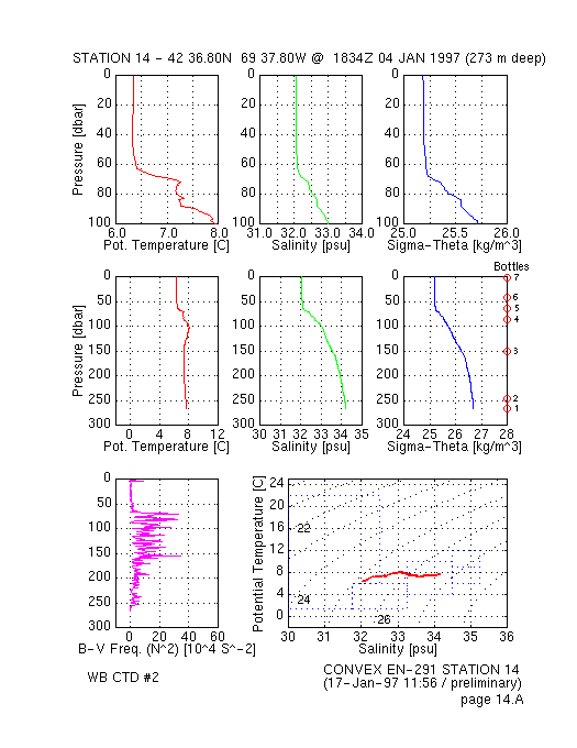
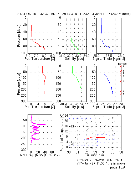
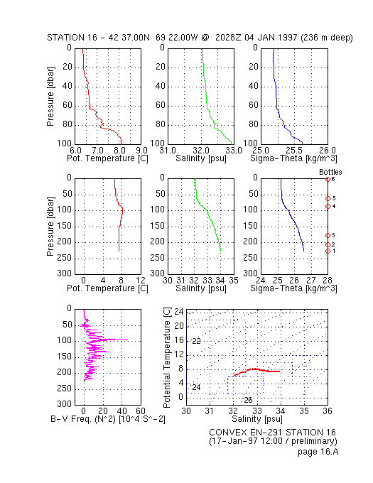
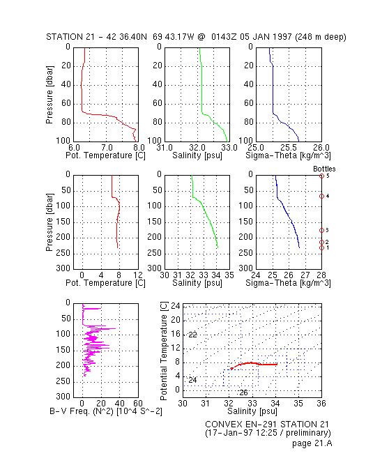
For each of the CTD stations, page "A" presents a set of profiles (potential temperature, salinity, sigma-theta)
and potential temperature-salinity diagrams (Figures 02A-29A). The upper surface to 100 m deep plots represent
zoomed details of water property structure in the main thermocline (halocline, pycnocline) zone (horizontal scales
vary). The middle plots present these water property structures for the entire water column (scales are fixed).
A Brunt-Vaisaila frequency (N-squared) plot indicates water column stability.
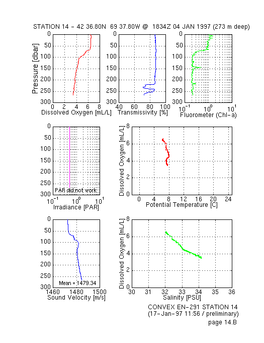
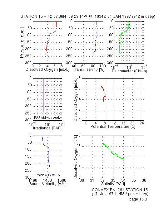
On page "B" are presented CTD station profiles of measured dissolved oxygen, Transmissivity, fluorometer (Chl-a),
irradiance (PAR), as well as computed sound velocity, temperature - dissolved oxygen, and salinity - dissolved
oxygen diagrams (Figures 02B-29B).
3.d.2. Vertical Sections:
Potential temperature, salinity, and sigma-theta sections for two transects are presented for:
- Waypoints A to F, tracking southeastward through Jeffreys and Wilkinson Basins
(Figure 5.a), and
- Waypoints B to G, tracking eastward through Massachusetts Bay and Wilkinson Basin
(Figure 5.b).
Contour intervals are 0.5 degC for temperature, 0.20 psu for salinity and 0.20 kg/cubic m for sigma-theta.
The CTD station numbers are indicated along the top horizontal axis and the ocean bottom is shaded.
3.d.3. Horizontal Layer Contours:
Representative hydrographic structures of the survey region are depicted by MATLAB contours of properties using
an inverse distance method. Grid resolution is 2 km. Extrapolation beyond the survey corners is masked out.
The WB-98 mooring position is marked.
3.d.3. Data Files
CTD Profiles are available immediately via ftp procedures at:
- "ftp ekman.sr.unh.edu"
- login as "anonymous" with your user name as the password
- change directory using "cd /pub/CONVEX/en291"
- read the README_CTD.FMT file for info on format, etc.
- download using normal "mget" procedures.
Please be aware that these are PROPRIATORY DATA. We have yet to complete the NSF-funded
research associated with these data and reserve the right to initial publication. Please contact
us for further information.
Individual profile data ASCII files are also available individually by clicking on the numbers in
the appendix table below.
Other EN-291 Cruise data including enroute ADCP, TSAL, navigation, bathymetry and observed weather records
will also be made available upon further processing.
4. Acknowledgements
The valuable work of Ken Morey, Dan Howard and Karen Garrison resulted in the successful deployment of the
Wilkinson Basin buoy and hydrographic survey. We appreciate the efforts of the captain and crew of R/V ENDEAVOR
as they helped us conduct this field program. We are grateful for the help provided by T. Loder and A. Wang /
V. Pilon in processing the bottle salinities. F. Bub, W. Brown, and P. Mupparapu are supported by NSF Grant
OCE-9530249. L. C. Smith was instrumental in preparing this report.
5. References
Fofonoff, N. P. and R. C. Millard Jr., 1983. Algorithms for compilation of fundamental properties of seawater,
UNESCO Technical Papers in Marine Science, no. 44. UNESCO, Paris, France, 53 pages.
Garrison, K. M. and W. S. Brown, 1989. Hydrographic survey in the Gulf of Maine July-August 1987, UNH Tech.
Rpt. No. UNHMP-T/DR-SG-89-5, Univ. of NH, Durham, NH.
Morgan, P. P., 1994, SEAWATER Software Version 1.2b, CSIRO Division of Oceanography, Hobart, AUS.
CTD station information for the R/V ENDEAVOR Cruise EN-291 (3-5 January 1997). Position, depth, date, and time
are for the bottom of the cast. The stations at the Wilkinson Basin (WB) and Jeffreys Basin (JB) mooring sites,
as well as three Massachusetts Water Resource Authority (MWRA) sites (F/N##) are indicated. Profile data, as
described above (3.d.1.), may be viewed by clicking on the CTD number. See Figure 1
for station locations. An ASCII listing of the CTDs is also available.
 CTD station    Latitude    Longitude   Water Depth  Time     Date
   number      (deg min N)  (deg min W)  (meters)    (Z)   (DD/MM/YY)
________________________________________________________________________

    02          42  39.47    69  42.02      265      22:04   03/01/97
    03          42  42.46    69  46.03      244      00:30   04/01/97
    04          42  45.65    69  50.46      234      01:58   04/01/97
    05          42  48.38    69  54.33      222      02:50   04/01/97
    06          42  51.53    69  58.60      204      03:46   04/01/97
    07          42  54.53    70  02.94      107      04:36   04/01/97
    08      JB1 42  57.57    70  07.93      138      05:23   04/01/97
    09          42  59.99    70  11.96      173      06:13   04/01/97
    10          43  02.95    70  16.12      161      07:01   04/01/97
    11          43  05.97    70  20.36      118      07:48   04/01/97
    12          43  09.00    70  24.53       80      08:34   04/01/97
    13          42  46.96    69  44.88      270      12:40   04/01/97
    14      WB1 42  36.80    69  37.80      273      18:34   04/01/97
    15          42  37.06    69  29.14      242      19:34   04/01/97
    16          42  37.00    69  22.00      236      20:28   04/01/97
    17          42  31.04    69  21.97      230      21:30   04/01/97
    18          42  25.13    69  22.01      252      22:34   04/01/97
    19          42  31.09    69  29.10      279      23:38   04/01/97
    20      WB2 42  36.47    69  37.65      274      00:50   05/01/97
    21          42  36.40    69  43.17      248      01:43   05/01/97
    22          42  35.94    69  48.59      266      02:29   05/01/97
    23          42  35.58    69  54.04      185      03:15   05/01/97
    24          42  34.70    70  05.01      110      04:25   05/01/97
    25          42  33.80    70  15.83       78      05:27   05/01/97
    26          42  33.34    70  21.38      102      06:05   05/01/97
    27      F27 42  33.01    70  26.70      106      06:46   05/01/97
    28      F22 42  28.83    70  37.00       81      07:58   05/01/97
    29      N16 42  23.66    70  45.14       45      09:09   05/01/97